Hypot

Description:
Calculates the length of the hypotenuse of a right-angled triangle given the lengths of the other two sides.This method computes z = Sqrt(Pow(x, 2) + Pow(y, 2)) by avoiding underflow and overflow.

\[\text{hypot}(x,y) = \sqrt{x^2 + y^2}\]
double Hypot(double x, double y)
ColVec Hypot(ColVec x, double y)
ColVec Hypot(double x, ColVec y)
RowVec Hypot(RowVec x, double y)
RowVec Hypot(double x, RowVec y)
Matrix Hypot(Matrix x, double y)
Matrix Hypot(double x, Matrix y)
ColVec Hypot(ColVec x, ColVec y)
RowVec Hypot(RowVec x, RowVec y)
Matrix Hypot(Matrix x, Matrix y)
Matrix Hypot(RowVec x, ColVec y)
Matrix Hypot(ColVec x, RowVec y)
Matrix Hypot(RowVec x, Matrix y)
Matrix Hypot(Matrix x, RowVec y)
Matrix Hypot(Matrix x, ColVec y)
Matrix Hypot(ColVec x, Matrix y)
Param:

x: The length of one side of the triangle.

y: The length of the other side of the triangle.

Returns:
The length of the hypotenuse.

Example:
Compute the hypotenus of a triangle with sides 3 and 4
var hypotenuse = Hypot(3, 4);
Console.WriteLine(hypotenuse);
Output:
5
Example:
Compute the hypotenus of a triangle with sides $[2,3,4,5]$ and $[7,6]^T$
RowVec X = new double[]{2,3,4,5};
ColVec Y = new double[]{7,6};
var hypotenuse = Hypot(X, Y);
Console.WriteLine(hypotenuse);
Output:
7.2801    7.6158    8.0623    8.6023
6.3246    6.7082    7.2111    7.8102

decic

Description:
Compute consistent initial conditions for ODE45I.

Param:

fun: The function that represents the implicit ODE. The function should accept three doubles (time, state, and its derivative) and return a double representing the derivative of the state.

t0: An array of time points at which the solution is desired. The first element is the initial time, and the last element is the final time.

y0: The initial value of the dependent variable (state).

ytruth: An array of intergers indicating which component of y0 is fixed and which is not.

yp0: The initial time derivative of the dependent variable (state).

yptruth: An array of intergers indicating which component yp0 is fixed and which is not.

options: Optional parameters for the ODE solver, such as relative tolerance, absolute tolerance, and maximum step size. If not provided, default options will be used.

Returns:

A tuple containing two elements:

double y0: modified initial state.

double yp0: modified initial rate of change.

Remark:

decic changes as few components of the guess as possible. You can specify that certain components are to be held fixed by setting ytruth(i) = 1 if no change is permitted

in the guess for Y0(i) and 0 otherwise.An empty array for yptruth is interpreted as allowing changes in all entries.yptruth is handled similarly.

You cannot fix more than length(Y0) components.Depending on the problem, it may not be possible to fix this many.It also may not be possible to fix certain components of Y0 or YP0.

It is recommended that you fix no more components than necessary.

Example:
Determine the consistent initial condition for the implicit ODE $~ty^2y'^3 - y^3y'^2 + t(t^2 + 1)y' - t^2y = 0~$ with initial condition $~y(0) = \sqrt{1.5}~$.
// import libraries
using System;
using SepalSolver.Math;

//define ODE
static double fun(double t, double y, double yp) =>
   t * y * y * yp * yp * yp - y * y * y * yp * yp + t * (t * t + 1) * yp - t * t * y;
   var opts = Odeset(Stats: true);
   double t0 = 1, y0 = Sqrt(t0 * t0 + 1 / 2.0), yp0 = 0;
   (y0, yp0) = decic(fun, t0, y0, 1, yp0, 0);

// print result to console
Console.WriteLine($"y0 = {y0}");
Console.WriteLine($"yp0 = {yp0}");
Output:
y0 = 1.2247
yp0 = 0.8165

cref=System.ArgumentNullException is Thrown when the dydx is null.

cref=System.ArgumentException is Thrown when the tspan array has less than two elements.

Ode23

Description:
Solves non stiff ordinary differential equations (ODE) using the Bogacki-Shampine method (Ode23).

Param:

dydx: The function that represents the ODE. The function should accept two doubles (time and state) and return a double representing the derivative of the state.

initcon: The initial value of the dependent variable (state).

tspan: An array of time points at which the solution is desired. The first element is the initial time, and the last element is the final time.

options: Optional parameters for the ODE solver, such as relative tolerance, absolute tolerance, and maximum step size. If not provided, default options will be used.

Returns:

A tuple containing two elements:

ColVec T: A column vector of time points at which the solution was computed.

Matrix Y: A matrix where each row corresponds to the state of the system at the corresponding time point in T.

Remark:

This method uses the Bogacki-Shampine method (Ode23) to solve the ODE. It is an adaptive step size method that adjusts the step size to achieve the desired accuracy.

For best results, the function should be smooth within the integration interval.

Example:
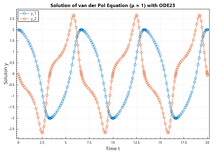
Solve the ODE $~d^2y/dt^2 = (1 - y^2)y' - y~$ with initial condition $~y(0) = [2, 0]~$ over the interval $[0, 2]$. First we have to convert this to a system of first order differential equations,

\[\begin{split}\begin{array}{rcl} y' &=& v \\ v' &=& (1 - y^2)v - y \end{array}\end{split}\]
// import libraries
using System;
using SepalSolver.Math;

//define ODE
static ColVec vdp1(double t, ColVec y)
{
     double[] dy;
     return dy = [y[1], (1 - y[0] * y[0]) * y[1] - y[0]];
}
//Solve ODE
(ColVec T, Matrix Y) = Ode23(vdp1, [2, 0], [0, 20]);
// Plot the result
Plot(T, Y, "-o");
Xlabel("Time t"); Ylabel("Soluton y");
Legend(["y_1", "y_2"], Alignment.UpperLeft);
Title("Solution of van der Pol Equation (μ = 1) with ODE23");
SaveAs("Van-der-Pol-(μ=1)-Ode23.png");
Output:

cref=System.ArgumentNullException is Thrown when the dydx is null.

cref=System.ArgumentException is Thrown when the tspan array has less than two elements.

Ode45

Description:
Solves non stiff ordinary differential equations (ODE) using the Dormand-Prince method (Ode45).

Param:

dydx: The function that represents the ODE. The function should accept two doubles (time and state) and return a double representing the derivative of the state.

initcon: The initial value of the dependent variable (state).

tspan: An array of time points at which the solution is desired. The first element is the initial time, and the last element is the final time.

options: Optional parameters for the ODE solver, such as relative tolerance, absolute tolerance, and maximum step size. If not provided, default options will be used.

Returns:

A tuple containing two elements:

ColVec T: A column vector of time points at which the solution was computed.

Matrix Y: A matrix where each row corresponds to the state of the system at the corresponding time point in T.

Remark:

This method uses the Dormand-Prince method (Ode45) to solve the ODE. It is an adaptive step size method that adjusts the step size to achieve the desired accuracy.

For best results, the function should be smooth within the integration interval.

Example:
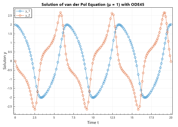
Solve the ODE $~d^2y/dt^2 = (1 - y^2)y' - y~$ with initial condition $~y(0) = [2, 0]~$ over the interval $[0, 2]$. First we have to convert this to a system of first order differential equations,

\[\begin{split}\begin{array}{rcl} y' &=& v \\ v' &=& (1 - y^2)v - y \end{array}\end{split}\]
// import libraries
using System;
using SepalSolver.Math;

//define ODE
static ColVec vdp1(double t, ColVec y)
{
     double[] dy;
     return dy = [y[1], (1 - y[0] * y[0]) * y[1] - y[0]];
}
//Solve ODE
(ColVec T, Matrix Y) = Ode45(vdp1, [2, 0], [0, 20]);
// Plot the result
Plot(T, Y, "-o");
Xlabel("Time t"); Ylabel("Soluton y");
Legend(["y_1", "y_2"], Alignment.UpperLeft);
Title("Solution of van der Pol Equation (μ = 1) with ODE45");
SaveAs("Van-der-Pol-(μ=1)-Ode45.png");
Output:

cref=System.ArgumentNullException is Thrown when the dydx is null.

cref=System.ArgumentException is Thrown when the tspan array has less than two elements.

Ode56

Description:
Solves non stiff ordinary differential equations (ODE) using the Jim Verner 5th and 6th order pair method (Ode56).

Param:

dydx: The function that represents the ODE. The function should accept two doubles (time and state) and return a double representing the derivative of the state.

initcon: The initial value of the dependent variable (state).

tspan: An array of time points at which the solution is desired. The first element is the initial time, and the last element is the final time.

options: Optional parameters for the ODE solver, such as relative tolerance, absolute tolerance, and maximum step size. If not provided, default options will be used.

Returns:

A tuple containing two elements:

ColVec T: A column vector of time points at which the solution was computed.

Matrix Y: A matrix where each row corresponds to the state of the system at the corresponding time point in T.

Remark:

This method uses the Jim Verner 5th and 6th order pair method (Ode56) to solve the ODE. It is an adaptive step size method that adjusts the step size to achieve the desired accuracy.

For best results, the function should be smooth within the integration interval.

Example:
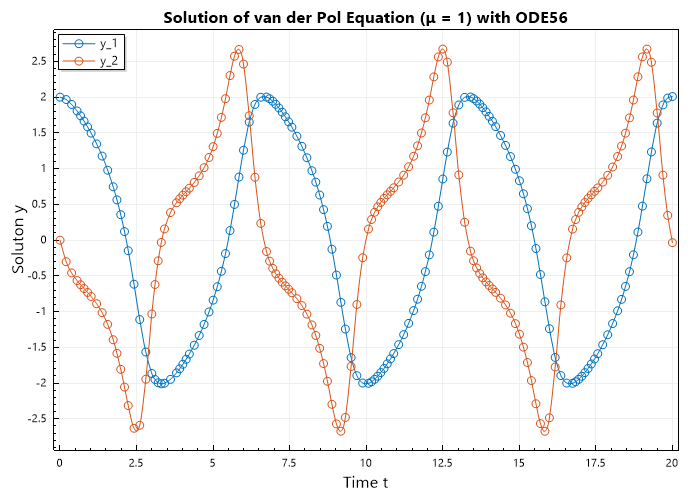
Solve the ODE $~d^2y/dt^2 = (1 - y^2)y' - y~$ with initial condition $~y(0) = [2, 0]~$ over the interval $[0, 20]$. First we have to convert this to a system of first order differential equations,

\[\begin{split}\begin{array}{rcl} y' &=& v \\ v' &=& (1 - y^2)v - y \end{array}\end{split}\]
// import libraries
using System;
using SepalSolver.Math;

//define ODE
static ColVec vdp1(double t, ColVec y)
{
     double[] dy;
     return dy = [y[1], (1 - y[0] * y[0]) * y[1] - y[0]];
}
//Solve ODE
(ColVec T, Matrix Y) = Ode56(vdp1, [2, 0], [0, 20]);
// Plot the result
Plot(T, Y, "-o");
Xlabel("Time t"); Ylabel("Soluton y");
Legend(["y_1", "y_2"], Alignment.UpperLeft);
Title("Solution of van der Pol Equation (μ = 1) with ODE56");
SaveAs("Van-der-Pol-(μ=1)-Ode56.png");
Output:

cref=System.ArgumentNullException is Thrown when the dydx is null.

cref=System.ArgumentException is Thrown when the tspan array has less than two elements.

Ode78

Description:
Solves non stiff ordinary differential equations (ODE) using the Jim Verner 7th and 8th order pair method (Ode78).

Param:

dydx: The function that represents the ODE. The function should accept two doubles (time and state) and return a double representing the derivative of the state.

initcon: The initial value of the dependent variable (state).

tspan: An array of time points at which the solution is desired. The first element is the initial time, and the last element is the final time.

options: Optional parameters for the ODE solver, such as relative tolerance, absolute tolerance, and maximum step size. If not provided, default options will be used.

Returns:

A tuple containing two elements:

ColVec T: A column vector of time points at which the solution was computed.

Matrix Y: A matrix where each row corresponds to the state of the system at the corresponding time point in T.

Remark:

This method uses the Jim Verner 7th and 8th order pair method (Ode78) to solve the ODE. It is an adaptive step size method that adjusts the step size to achieve the desired accuracy.

For best results, the function should be smooth within the integration interval.

Example:
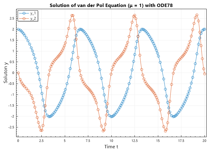
Solve the ODE $~d^2y/dt^2 = (1 - y^2)y' - y~$ with initial condition $~y(0) = [2, 0]~$ over the interval $[0, 20]$. First we have to convert this to a system of first order differential equations,

\[\begin{split}\begin{array}{rcl} y' &=& v \\ v' &=& (1 - y^2)v - y \end{array}\end{split}\]
// import libraries
using System;
using SepalSolver.Math;

//define ODE
static ColVec vdp1(double t, ColVec y)
{
     double[] dy;
     return dy = [y[1], (1 - y[0] * y[0]) * y[1] - y[0]];
}
//Solve ODE
(ColVec T, Matrix Y) = Ode78(vdp1, [2, 0], [0, 20]);
// Plot the result
Plot(T, Y, "-o");
Xlabel("Time t"); Ylabel("Soluton y");
Legend(["y_1", "y_2"], Alignment.UpperLeft);
Title("Solution of van der Pol Equation (μ = 1) with ODE78");
SaveAs("Van-der-Pol-(μ=1)-Ode78.png");
Output:

cref=System.ArgumentNullException is Thrown when the dydx is null.

cref=System.ArgumentException is Thrown when the tspan array has less than two elements.

Ode89

Description:
Solves non stiff ordinary differential equations (ODE) using the Jim Verner 8th and 9th order pair method (Ode89).

Param:

dydx: The function that represents the ODE. The function should accept two doubles (time and state) and return a double representing the derivative of the state.

initcon: The initial value of the dependent variable (state).

tspan: An array of time points at which the solution is desired. The first element is the initial time, and the last element is the final time.

options: Optional parameters for the ODE solver, such as relative tolerance, absolute tolerance, and maximum step size. If not provided, default options will be used.

Returns:

A tuple containing two elements:

ColVec T: A column vector of time points at which the solution was computed.

Matrix Y: A matrix where each row corresponds to the state of the system at the corresponding time point in T.

Remark:

This method uses the Jim Verner 8th and 9th order pair method (Ode89) to solve the ODE. It is an adaptive step size method that adjusts the step size to achieve the desired accuracy.

For best results, the function should be smooth within the integration interval.

Example:
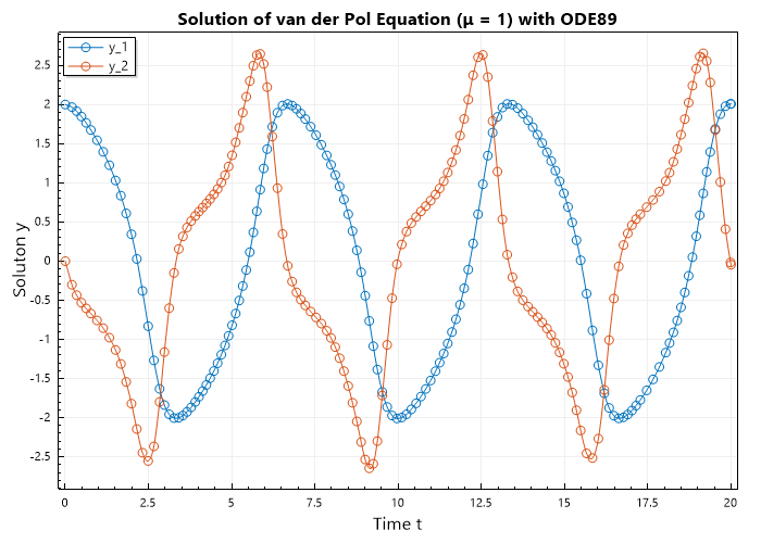
Solve the ODE $~d^2y/dt^2 = (1 - y^2)y' - y~$ with initial condition $~y(0) = [2, 0]~$ over the interval $[0, 20]$. First we have to convert this to a system of first order differential equations,

\[\begin{split}\begin{array}{rcl} y' &=& v \\ v' &=& (1 - y^2)v - y \end{array}\end{split}\]
// import libraries
using System;
using SepalSolver.Math;

//define ODE
static ColVec vdp1(double t, ColVec y)
{
     double[] dy;
     return dy = [y[1], (1 - y[0] * y[0]) * y[1] - y[0]];
}
//Solve ODE
(ColVec T, Matrix Y) = Ode89(vdp1, [2, 0], [0, 20]);
// Plot the result
Plot(T, Y, "-o");
Xlabel("Time t"); Ylabel("Soluton y");
Legend(["y_1", "y_2"], Alignment.UpperLeft);
Title("Solution of van der Pol Equation (μ = 1) with ODE89");
SaveAs("Van-der-Pol-(μ=1)-Ode89.png");
Output:

cref=System.ArgumentNullException is Thrown when the dydx is null.

cref=System.ArgumentException is Thrown when the tspan array has less than two elements.

Ode45s

Description:
Solves stiff ordinary differential equations (ODE) using Adaptive Diagonally Implicit RungeKutta of 4th and 5th Order Method (Ode45s).

Param:

dydx: The function that represents the ODE. The function should accept two doubles (time and state) and return a double representing the derivative of the state.

initcon: The initial value of the dependent variable (state).

tspan: An array of time points at which the solution is desired. The first element is the initial time, and the last element is the final time.

options: Optional parameters for the ODE solver, such as relative tolerance, absolute tolerance, and maximum step size. If not provided, default options will be used.

Returns:

A tuple containing two elements:

ColVec T: A column vector of time points at which the solution was computed.

Matrix Y: A matrix where each row corresponds to the state of the system at the corresponding time point in T.

Remark:

This method uses Adaptive Diagonally Implicit RungeKutta of 4th and 5th Order Method (Ode45s) to solve the ODE. It is an adaptive step size method that adjusts the step size to achieve the desired accuracy.

For best results, the function should be smooth within the integration interval.

Example:
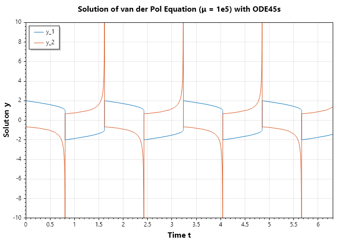
Solve the ODE $~d^2y/dt^2 = 10^{5}((1 - y^2)y' - y)~$ with initial condition $~y(0) = [2, 0]~$ over the interval $[0, 6.3]$. First we have to convert this to a system of first order differential equations,

\[\begin{split}\begin{array}{rcl} y' &=& v \\ v' &=& 10^{5}((1 - y^2)v - y) \end{array}\end{split}\]
// import libraries
using System;
using SepalSolver.Math;

//define ODE
static ColVec vdp2(double t, ColVec y)
{
     double[] dy;
     return dy = [y[1], 1e5*((1 - y[0] * y[0]) * y[1] - y[0])];
}
//Solve ODE
(ColVec T, Matrix Y) = Ode45s(vdp2, [2, 0], [0, 6.3]);
// Plot the result
Plot(T, Y);
Xlabel("Time t"); Ylabel("Soluton y");
Legend(["y_1", "y_2"], Alignment.UpperLeft);
Title("Solution of van der Pol Equation (μ = 1e5) with ODE45s");
SaveAs("Van-der-Pol-(μ=1e5)-Ode45s");
Output:

cref=System.ArgumentNullException is Thrown when the dydx is null.

cref=System.ArgumentException is Thrown when the tspan array has less than two elements.

Ode45i

Description:
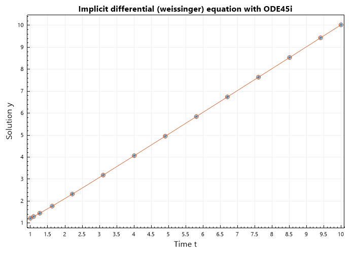
Solves inmplicit ordinary differential equations (ODE) using Adaptive Diagonally Implicit RungeKutta of 4th and 5th Order Method (Ode45i).

Param:

fun: The function that represents the implicit ODE. The function should accept three doubles (time, state, and its derivative) and return a double representing the derivative of the state.

initcon: A tuple containing two elements: * double y0: initial state. * double yp0: initial rate of change.

tspan: The initial value of the dependent variable (state).

options: Optional parameters for the ODE solver, such as relative tolerance, absolute tolerance, and maximum step size. If not provided, default options will be used.

Returns:

A tuple containing two elements:

ColVec T: A column vector of time points at which the solution was computed.

Matrix Y: A matrix where each row corresponds to the state of the system at the corresponding time point in T.

Remark:

This method uses Adaptive Diagonally Implicit RungeKutta of 4th and 5th Order Method (Ode45i) to solve the ODE. It is an adaptive step size method that adjusts the step size to achieve the desired accuracy.

For best results, the function should be smooth within the integration interval.

Example:
Solve the ODE $~ty^2y'^3 - y^3y'^2 + t(t^2 + 1)y' - t^2y = 0~$ with initial condition $~y(0) = \sqrt{1.5}~$.
// import libraries
using System;
using SepalSolver.Math;

//define ODE
static double fun(double t, double y, double yp) =>
   t* y * y* yp * yp* yp - y* y * y* yp * yp + t* (t* t + 1) * yp - t* t * y;

var opts = Odeset(Stats: true);
double t0 = 1, y0 = Sqrt(t0 * t0 + 1 / 2.0), yp0 = 0;
(y0, yp0) = decic(fun, t0, y0, 1, yp0, 0);
(ColVec T, Matrix Y) = Ode45i(fun, (y0, yp0), [t0, 10], opts);
ColVec Y_exact = T.Select(t => Sqrt(t * t + 0.5)).ToList();
Console.WriteLine(Hcart(Y, Y_exact));
Plot(T, Y, "*"); hold = true;
Plot(T, Y_exact, "-o"); hold = false;
Title("Implicit differential (weissinger) equation with ODE45i");
Xlabel("Time t");
Ylabel("Solution y");
SaveAs("Weissinger-Ode45i.png");
Output:
Summary of statistics by Ode45i

13 successful steps 0 failed attempts 335 function evaluations 52 partial derivatives 52 LU decompositions 174 solutions of linear systems

1.2247 1.2247 1.2993 1.2993 1.4536 1.4536 1.7767 1.7768 2.3227 2.3229 3.1865 3.1869 4.0689 4.0694 4.9575 4.9582 5.8496 5.8504 6.7437 6.7447 7.6392 7.6403 8.5357 8.5368 9.4327 9.4340

10.0236 10.0250
Output:

cref=System.ArgumentNullException is Thrown when the dydx is null.

cref=System.ArgumentException is Thrown when the tspan array has less than two elements.

Polyfit

Description:
Fits a polynomial of degree N to the data points specified by the arrays X and Y. Mathematically, this can be represented as finding the coefficients of the polynomial:

\[P(x) = a_0 + a_1 x + a_2 x^2 + ... + a_N x^N\]

that best fits the given data points (X, Y).

Param:

X: The x-coordinates of the data points.

Y: The y-coordinates of the data points.

N: The degree of the polynomial to fit.

Returns:
An array containing the coefficients of the fitted polynomial, starting with the coefficient of the highest degree term.

Example:
\[X = [1, 2, 3, 4],~ Y = [1, 4, 9, 16],~ N = 2\]

In this example, we fit a polynomial of degree 2 to the data points. The x-coordinates are represented by the array { 1, 2, 3, 4 } and the y-coordinates by { 1, 4, 9, 16 }.
// import libraries
using System;
using SepalSolver.Math;

// Example of fitting a polynomial
double[] X = { 1, 2, 3, 4 };
double[] Y = { 1, 4, 9, 16 };
int N = 2;
double[] coefficients = Polyfit(X, Y, N);
// Print the result
Console.WriteLine($"Coefficients: {string.Join(", ", coefficients)}");
Output:
Coefficients: 1, 0, 0

Roots

Description:
Calculates the roots of a polynomial given its coefficients. Mathematically, this can be represented as:

\[P(x) = 0\]

where P(x) is the polynomial.
Complex[] Roots(double[] Coeffs)
Complex[] Roots(Complex[] Coeffs)
Param:

Coeffs: The coefficients of the polynomial, ordered from the highest degree to the constant term.

Returns:
An array of Complex numbers representing the roots of the polynomial.
Example:
\[P(x) = 2x^5 + 3x^4 + 5x^3 + 2x^2 + 7x + 4\]

In this example, we find the roots of the polynomial represented by the coefficients { 2, 3, 4, 2, 7, 4 }.
// import libraries
using System;
using SepalSolver;
using static SepalSolver.Math;

// Example of finding roots of a polynomial
double[] Coeffs = [2, 3, 4, 2, 7, 4];
Complex[] roots = Roots(Coeffs);
// Print the result
Console.WriteLine($"Roots:\n {string.Join("\n ", roots)}");
Output:
Roots:
  -0.5854 + 0.0000i
   0.5737 - 1.0415i
   0.5737 + 1.0415i
  -1.0310 - 1.1635i
  -1.0310 + 1.1635i
..note::
The coefficients can be real or complex.

Example:
\[\begin{array}{rcl} P(x) &=& (5 + 2i)x^4 + (3 + 7i)x^3 + (5 + 8i)x^2 + (3 + 7i)x + (7 + 4i) \end{array}\]

In this example, we find the roots of the polynomial with complex coefficients.
// import libraries
using System;
using SepalSolver;
using static SepalSolver.Math;

// Example of finding roots of a polynomial with complex coefficients
Complex[] Coeffs = [new(5, 2), new(3, 7), new(5, 8), new(3, 7), new(7, 4)];
Complex[] roots = Roots(Coeffs);

// Print the result
Console.WriteLine($"Roots:\n {string.Join("\n ", roots)}");
Output:
Roots:
   0.2097 + 0.7705i
  -0.7572 + 0.6704i
  -0.7626 - 0.9963i
   0.3102 - 1.4446i

Deconv

Description:
Performs polynomial deconvolution (division) of two polynomials and returns the quotient and remainder. Mathematically, this can be represented as:

\[P(x) = D(x) \times Q(x) + R(x)\]

where P(x) is the dividend polynomial, D(x) is the divisor polynomial, Q(x) is the quotient polynomial, and R(x) is the remainder polynomial.
(double[] Quotient, double[] Remainder) Deconv(double[] Polynomial, double[] Divisor)
(Complex[] Quotient, Complex[] Remainder) Deconv(Complex[] Polynomial, Complex[] Divisor)
Param:

Polynomial: The coefficients of the dividend polynomial (numerator).

Divisor: The coefficients of the divisor polynomial (denominator).

Returns:

A tuple containing two arrays:

Quotient: The coefficients of the quotient polynomial.

Remainder: The coefficients of the remainder polynomial.
Example:
\[P(x) = x^5 + 2x^4 + 3x^3 + 4x^2 + 5x + 6,~ D(x) = x^2 + 2x + 3\]

In this example, we perform polynomial deconvolution on two polynomials. The dividend polynomial is represented by the coefficients { 1, 2, 3, 4, 5, 6 } and the divisor polynomial by { 1, 2, 3 }.
// import libraries
using System;
using SepalSolver.Math;

// Example of performing polynomial deconvolution
double[] Polynomial = [1, 2, 3, 4, 5, 6];
double[] Divisor = [1, 2, 3];
var result = Deconv(Polynomial, Divisor);
// Print the result
Console.WriteLine($"Quotient: {string.Join(", ", result.Quotient)}");
Console.WriteLine($"Remainder: {string.Join(", ", result.Remainder)}");
Output:
Quotient: 1, 0, 0, 4
Remainder: 0, 0, 0, 0, -3, -6
..note::
Both polynomial and the divisor can be real or complex as demonstrated below

Example:
\[\begin{split}\begin{array}{rcl} P(x) &=& (7+3i)x^3 + (9+10i)x^2 + (10+4i)x + (2+7i) \\ D(x) &=& (3+2i)x^2 + (4+2i)x + (3+i) \end{array}\end{split}\]

In this example, we perform polynomial deconvolution on two polynomials with complex coefficients.
// import libraries
using System;
using SepalSolver.Math;

// Example of performing polynomial deconvolution
Complex[] P = [new(7,3), new(9,10), new(10,4), new(2,7)],
Complex[] D = [new(3,2), new(4,2), new(3,1)];
(Complex[]Q, Complex[]R) = Deconv(P, D);

// Print the result
Console.WriteLine("Q = \n" + string.Join(", ", Q));
Console.WriteLine("R = \n" + string.Join(", ", R));
Output:
Q =
    2.0769 - 0.3846i ,  1.1183 + 1.7160i
R =
    0.0000 + 0.0000i ,  0.0000 + 0.0000i ,  2.3432 - 6.0237i ,  0.3609 + 0.7337i

Conv

Description:
Performs polynomial convolution (multiplication) of two polynomials and returns the resulting polynomial. Mathematically, this can be represented as:

\[C(x) = P(x) \times M(x)\]

where P(x) is the first polynomial, M(x) is the second polynomial, and C(x) is the resulting polynomial.
double[] Conv(double[] Polynomial, double[] Multiplier)
Complex[] Conv(Complex[] Polynomial, Complex[] Multiplier)
Param:

Polynomial: The coefficients of the first polynomial.

Multiplier: The coefficients of the second polynomial.

Returns:
An array containing the coefficients of the resulting polynomial.
Example:
\[P(x) = x^2 + 2x + 3,~ M(x) = x + 1\]

In this example, we perform polynomial convolution on two polynomials. The first polynomial is represented by the coefficients $[1, 2, 3]$ and the second polynomial by $[1, 1]$.
// import libraries
using System;
using SepalSolver.Math;

// Example of performing polynomial convolution
double[] Polynomial = [ 1, 2, 3 ];
double[] Multiplier = [ 1, 1 ];
double[] Product = Conv(Polynomial, Multiplier);
// Print the result
Console.WriteLine($"Product: {string.Join(", ", Product)}");
Output:
Product: 1, 3, 5, 3
Example:
\[P(x) = (2+3i)x^2 + (5-i)x + 3+7i,~ M(x) = (-3+2i)x + 2-i\]

In this example, we perform polynomial convolution on two polynomials. The first polynomial is represented by the coefficients $[2+3i, 5-i, 3+7i]$ and the second polynomial by $[-3+2i, 2-i]$.
// import libraries
using System;
using SepalSolver.Math;

// Example of performing polynomial convolution
Complex[] Polynomial = [ new(2,3), new(5,-1), new(3,7) ];
Complex[] Multiplier = [ new(-3,2), new(2,-1) ];
var Product = Conv(Polynomial, Multiplier);
// Print the result
Console.WriteLine($"Product: {string.Join(", ", Product)}");
Output:
Product: -12 - 5i ,  -6 + 17i, -14 - 22i,  13 + 11i

Integral

Description:
Computes the definite integral of a function using adaptive Gauss-LegendreP quadrature.

Param:

fun: The function to integrate. The function should accept a double and return a double.

x_1: The lower bound of the integration interval.

x_2: The upper bound of the integration interval.

eps: The desired relative accuracy. The default value is 1e-6.

Returns:
The approximate value of the definite integral.

Remark:

This method uses adaptive Gauss-LegendreP quadrature to approximate the definite integral.

The number of quadrature points is increased until the desired relative accuracy is achieved or a maximum number of iterations is reached.

For best results, the function should be smooth within the integration interval.

If x_1 equals x_2 then the method will return 0.

Example:
Integrate the function f(x) = x^2, which can be expressed as:

\[\int_{x_1}^{x_2} x^2 \, dx\]
// import libraries
using System;
using SepalSolver.Math;

// Define the function to integrate
Func<double, double> f = (x) => x * x;
// Set the lower bound of x
double x_1 = 0;
// Set the upper bound of x
double x_2 = 1;
// Calculate the integral
double integral = Integral(f, x_1, x_2);
// Print the result
Console.WriteLine($"The integral of x^2 is approximately: {integral}");
Output:
The integral of x^2 is approximately: 0.333333333321056

cref=System.ArgumentNullException is Thrown when the fun is null.

cref=System.Exception is Thrown when the maximum number of iterations is reached without achieving the desired accuracy.

Integral2

Description:
Computes the definite double integral of a function over a region where both y-bounds are defined by functions of x, using adaptive Gauss-LegendreP quadrature. Mathematically, this can be represented as:

\[I = \int_{x_1}^{x_2}\int_{y_1}^{y_2} f(x,y) dydx\]
double Integral2( Func<double, double, double> fun, double x_1, double x_2, double y_1, double y_2)
double Integral2( Func<double, double, double> fun, double x_1, double x_2, double y_1, Func<double, double> y_2)
double Integral2( Func<double, double, double> fun, double x_1, double x_2, Func<double, double> y_1, double y_2)
double Integral2( Func<double, double, double> fun, double x_1, double x_2, Func<double, double> y_1, Func<double, double> y_2)
Param:

fun: The function to integrate. The function should accept two doubles (x, y) and return a double.

x_1: The lower bound of the x integration.

x_2: The upper bound of the x integration.

y_1: A function that defines the lower bound of the y integration as a function of x. It should accept a double (x) and return a double (y).

y_2: A function that defines the upper bound of the y integration as a function of x. It should accept a double (x) and return a double (y).

eps: The desired relative accuracy. The default value is 1e-6.

Returns:
The approximate value of the definite double integral.

Remark:

This method uses adaptive Gauss-LegendreP quadrature to approximate the double integral.

The integration is performed over the region defined by x_1 <= x <= x_2 and y_1(x) <= y <= y_2(x).

The number of quadrature points is increased until the desired relative accuracy is achieved or a maximum number of iterations is reached.

For best results, the function should be smooth within the integration region, and both y_1(x) and y_2(x) should be smooth functions. Additionally, y_1(x) should be less than or equal to y_2(x) for all x in the interval [x_1, x_2] to ensure a valid integration region.

If x_1 equals x_2 then the method will return 0.

Example:
Integrate the function f(x, y) = x * y over the region where x ranges from 0 to 1, y ranges from x^2 to sqrt(x), which can be expressed as:

\[\int_{0}^{1} \int_{x^{2}}^{\sqrt{x}} x y \, dy \, dx\]
// import libraries
using System;
using SepalSolver.Math;

// Define the function to integrate
Func<double, double, double> f = (x, y) => x * y;
// Define the lower bound of y as a function of x
Func<double, double> y_1 = (x) => x * x;
// Define the upper bound of y as a function of x
Func<double, double> y_2 = (x) => Sqrt(x);
// Set the lower bound of x
double x_1 = 0;
// Set the upper bound of x
double x_2 = 1;
// Calculate the integral
double integral = Integral2(f, x_1, x_2, y_1, y_2);
// Print the result
Console.WriteLine($"The integral is approximately: {integral}");
Output:
The integral is approximately: 0.0833333333277262
..note::
If the any of the boundary of y is a constant, it can be defined as a lambda function that returns the constant value as shown below:

Example:
Integrate the function f(x, y) = x * y, which can be expressed as:

\[\int_{0}^{1} \int_{1}^{2} x y \, dy \, dx\]
// import libraries
using System;
using SepalSolver.Math;

// Define the function to integrate
Func<double, double, double> f = (x, y) => x * y;
// Set the lower bound of x
double x_1 = 0;
// Set the upper bound of x
double x_2 = 1;
// Set the lower bound of y
Func<double, double> y_1 = x => 1;
// Set the upper bound of y
Func<double, double> y_2 = x => 2;
// Calculate the integral
double integral = Integral2(f, x_1, x_2, y_1, y_2);
// Print the result
Console.WriteLine($"The integral of x*y is approximately: {integral}");
Output:
The integral of x*y is approximately: 0.749999999948747
Example:
Integrate the function f(x, y) = x * y over the region where x ranges from 0 to 1, and y ranges from x^2 to 2, which can be expressed as:

\[\int_{x_1}^{x_2} \int_{y_1(x)}^{y_2} x y \, dy \, dx\]
// import libraries
using SepalSolver;
using System;

// Define the function to integrate
Func<double, double, double> f = (x, y) => x * y;
// Define the lower bound of y as a function of x
Func<double, double> y_1 = (x) => x * x;
// Set the lower bound of x
double x_1 = 0;
// Set the upper bound of x
double x_2 = 1;
// Set the upper bound of y
double y_2 = 2;
// Calculate the integral
double integral = Integrators.GaussLeg2(f, x_1, x_2, y_1, y_2);
// Print the result
Console.WriteLine($"The integral is approximately: {integral}");
Output:
The integral is approximately: 0.916666666604556
Example:
Integrate the function f(x, y) = x * y over the region where x ranges from 0 to 1, and y ranges from 1 to x^2, which can be expressed as:

\[\int_{x_1}^{x_2} \int_{y_1}^{y_2(x)} x y \, dy \, dx\]
// import libraries
using SepalSolver;
using System;

// Define the function to integrate
Func<double, double, double> f = (x, y) => x * y;
// Define the upper bound of y as a function of x
Func<double, double> y_2 = (x) => x * x;
// Set the lower bound of x
double x_1 = 0;
// Set the upper bound of x
double x_2 = 1;
// Set the lower bound of y
double y_1 = 1;
// Calculate the integral
double integral = Integrators.GaussLeg2(f, x_1, x_2, y_1, y_2);
// Print the result
Console.WriteLine($"The integral is approximately: {integral}");
Output:
The integral is approximately: -0.166666666655809
Example:
Integrate the function f(x, y) = x * y over the region where x ranges from 0 to 1, y ranges from x^2 to sqrt(x), which can be expressed as:

\[\int_{x_1}^{x_2} \int_{y_1(x)}^{y_2(x)} x y \, dy \, dx\]
// import libraries
using SepalSolver;
using static System.Math
using System;

// Define the function to integrate
Func<double, double, double> f = (x, y) => x * y;
// Define the lower bound of y as a function of x
Func<double, double> y_1 = (x) => x * x;
// Define the upper bound of y as a function of x
Func<double, double> y_2 = (x) => Sqrt(x);
// Set the lower bound of x
double x_1 = 0;
// Set the upper bound of x
double x_2 = 1;
// Calculate the integral
double integral = Integrators.GaussLeg2(f, x_1, x_2, y_1, y_2);
// Print the result
Console.WriteLine($"The integral is approximately: {integral}");
Output:
The integral is approximately: 0.0833333333277262

cref=System.ArgumentNullException is Thrown when the  fun is null.
cref=System.ArgumentNullException is Thrown when the  y_1 is null.
cref=System.ArgumentNullException is Thrown when the  y_2 is null.
cref=System.ArgumentException is Thrown when y_1(x) is greater than y_2(x) for any x in the interval [x_1, x_2].

Integral3

Description:

Computes the definite triple integral of a function over a region where the y-bounds are defined by functions of x, and the z-bounds are defined by functions of x and y, using adaptive Gauss-LegendreP quadrature. Mathematically, this can be represented as:

\[I = \int_{x_1}^{x_2}\int_{y_1}^{y_2}\int_{z_1}^{z_2} f(x,y, z) dzdydx\]

double Integral3( Func<double, double, double, double> fun, double x_1, double x_2, double y_1, double y_2, double z_1, double z_2)
double Integral3( Func<double, double, double, double> fun, double x_1, double x_2, double y_1, Func<double, double> y_2, double z_1, double z_2)
double Integral3( Func<double, double, double, double> fun, double x_1, double x_2, Func<double, double> y_1, double y_2, double z_1, double z_2)
double Integral3( Func<double, double, double, double> fun, double x_1, double x_2, Func<double, double> y_1, Func<double, double> y_2, double z_1, double z_2)
double Integral3( Func<double, double, double, double> fun, double x_1, double x_2, double y_1, double y_2, Func<double, double, double> z_1, double z_2)
double Integral3( Func<double, double, double, double> fun, double x_1, double x_2, double y_1, Func<double, double> y_2, Func<double, double, double> z_1, double z_2)
double Integral3( Func<double, double, double, double> fun, double x_1, double x_2, Func<double, double> y_1, double y_2, Func<double, double, double> z_1, double z_2)
double Integral3( Func<double, double, double, double> fun, double x_1, double x_2, Func<double, double> y_1, Func<double, double> y_2, Func<double, double, double> z_1, double z_2)
double Integral3( Func<double, double, double, double> fun, double x_1, double x_2, double y_1, double y_2, double z_1, Func<double, double, double> z_2)
double Integral3( Func<double, double, double, double> fun, double x_1, double x_2, double y_1, Func<double, double> y_2, double z_1, Func<double, double, double> z_2)
double Integral3( Func<double, double, double, double> fun, double x_1, double x_2, Func<double, double> y_1, double y_2, double z_1, Func<double, double, double> z_2)
double Integral3( Func<double, double, double, double> fun, double x_1, double x_2, Func<double, double> y_1, Func<double, double> y_2, double z_1, Func<double, double, double> z_2)
double Integral3( Func<double, double, double, double> fun, double x_1, double x_2, double y_1, double y_2, Func<double, double, double> z_1, Func<double, double, double> z_2)
double Integral3( Func<double, double, double, double> fun, double x_1, double x_2, double y_1, Func<double, double> y_2, Func<double, double, double> z_1, Func<double, double, double> z_2)
double Integral3( Func<double, double, double, double> fun, double x_1, double x_2, Func<double, double> y_1, double y_2, Func<double, double, double> z_1, Func<double, double, double> z_2)
double Integral3( Func<double, double, double, double> fun, double x_1, double x_2, Func<double, double> y_1, Func<double, double> y_2, Func<double, double, double> z_1, Func<double, double, double> z_2)

Param:

fun:  The function to integrate. The function should accept three doubles (x, y, z) and return a double.
x_1:  The lower bound of the x integration.
x_2:  The upper bound of the x integration.
y_1:  A function that defines the lower bound of the y integration as a function of x. It should accept a double (x) and return a double (y).
y_2:  A function that defines the upper bound of the y integration as a function of x. It should accept a double (x) and return a double (y).
z_1:  A function that defines the lower bound of the z integration as a function of x and y. It should accept two doubles (x, y) and return a double (z).
z_2:  A function that defines the upper bound of the z integration as a function of x and y. It should accept two doubles (x, y) and return a double (z).
eps:  The desired relative accuracy. The default value is 1e-6.

Returns:

The approximate value of the definite triple integral.

Remark:

This method uses adaptive Gauss-LegendreP quadrature to approximate the triple integral.
The integration is performed over the region defined by x_1 <= x <= x_2, y_1(x) <= y <= y_2(x), and z_1(x, y) <= z <= z_2(x, y).
The number of quadrature points is increased until the desired relative accuracy is achieved or a maximum number of iterations is reached.
For best results, the function should be smooth within the integration region, y_1(x), y_2(x), z_1(x, y), and z_2(x, y) should be smooth functions.
Ensure that y_1(x) <= y_2(x) and z_1(x, y) <= z_2(x, y) throughout the integration region.
If x_1 equals x_2 then the method will return 0.

Example:

Integrate the function f(x, y, z) = x * y * z over the region where x ranges from 0 to 1, y ranges from 1 to 2, and z ranges from 2 to 3, which can be expressed as:

\[\int_{x_1}^{x_2} \int_{y_1}^{y_2} \int_{z_1}^{z_2} x y z \, dz \, dy \, dx\]

// import libraries
using SepalSolver;
using System;

// Define the function to integrate
Func<double, double, double, double> f = (x, y, z) => x * y * z;
// Set the lower bound of x
double x_1 = 0;
// Set the upper bound of x
double x_2 = 1;
// Set the lower bound of y
double y_1 = 1;
// Set the upper bound of y
double y_2 = 2;
// Set the lower bound of z
double z1 = 2;
// Set the upper bound of z
double z2 = 3;
// Calculate the integral
double integral = Integral3(f, x_1, x_2, y_1, y_2, z1, z2);
// Print the result
Console.WriteLine($"The triple integral of x*y*z is approximately: {integral}");

Output:

The triple integral of x*y*z is approximately: 1.8749999998078

<example>: Integrate the function f(x, y, z) = x * y * z over the region where x ranges from 0 to 1, y ranges from x^2 to sqrt(x), and z ranges from 2 to 3, which can be expressed as:

\[\int_{x_1}^{x_2} \int_{y_1(x)}^{y_2(x)} \int_{z_1}^{z_2} x y z \, dz \, dy \, dx\]

// import libraries
using SepalSolver;
using static System.Math
using System;

// Define the function to integrate
Func<double, double, double, double> f = (x, y, z) => x * y * z;
// Define the lower bound of y as a function of x
Func<double, double> y_1 = (x) => x * x;
// Define the upper bound of y as a function of x
Func<double, double> y_2 = (x) => Sqrt(x);
// Set the lower bound of z
double z_1 = 2;
// Set the upper bound of z
double z_2 = 3;
// Set the lower bound of x
double x_1 = 0;
// Set the upper bound of x
double x_2 = 1;
// Calculate the integral
double integral = Integral3(f, x_1, x_2, y_1, y_2, z_1, z_2);
// Print the result
Console.WriteLine($"The triple integral of x*y*z is approximately: {integral}");

Output:

The triple integral of x*y*z is approximately: 0.208333333312197

Example:

Integrate the function f(x, y, z) = x * y * z over the region where x ranges from 0 to 1, y ranges from 1 to x^2, and z ranges from 2 to 3, which can be expressed as:

\[\int_{x_1}^{x_2} \int_{y_1}^{y_2(x)} \int_{z_1}^{z_2} x y z \, dz \, dy \, dx\]

// import libraries
using SepalSolver;
using System;

// Define the function to integrate
Func<double, double, double, double> f = (x, y, z) => x * y * z;
// Define the upper bound of y as a function of x
Func<double, double> y_2 = (x) => x * x;
// Set the lower bound of x
double x_1 = 0;
// Set the upper bound of x
double x_2 = 1;
// Set the lower bound of y
double y_1 = 1;
// Set the lower bound of z
double z_1 = 2;
// Set the upper bound of z
double z_2 = 3;
// Calculate the integral
double integral = Integral3(f, x_1, x_2, y_1, y_2, z_1, z_2);
// Print the result
Console.WriteLine($"The triple integral of x*y*z is approximately: {integral}");

Output:

The triple integral of x*y*z is approximately: -0.416666666625285

Example:

Integrate the function f(x, y, z) = x * y * z over the region where x ranges from 0 to 1, y ranges from x^2 to 2, and z ranges from 2 to 3, which can be expressed as:

\[\int_{x_1}^{x_2} \int_{y_1(x)}^{y_2} \int_{z_1}^{z_2} x y z \, dz \, dy \, dx\]

// import libraries
using SepalSolver;
using System;

// Define the function to integrate
Func<double, double, double, double> f = (x, y, z) => x * y * z;
// Define the lower bound of y as a function of x
Func<double, double> y_1 = (x) => x * x;
// Set the upper bound of y
double y_2 = 2;
// Set the lower bound of z
double z_1 = 2;
// Set the upper bound of z
double z_2 = 3;
// Set the lower bound of x
double x_1 = 0;
// Set the upper bound of x
double x_2 = 1;
// Calculate the integral
double integral = Integral3(f, x_1, x_2, y_1, y_2, z_1, z_2);
// Print the result
Console.WriteLine($"The triple integral of x*y*z is approximately: {integral}");

Output:

The triple integral of x*y*z is approximately: 2.29166666643309

Example:

Integrate the function f(x, y, z) = x * y * z over the region where x ranges from 0 to 1, y ranges from x^2 to sqrt(x), and z ranges from x*y to x+y, which can be expressed as:

\[\int_{0}^{1} \int_{x^{2}}^{\sqrt{x}} \int_{xy}^{x+y} x y z \, dz \, dy \, dx\]

// import libraries
using System;
using SepalSolver.Math;

// Define the function to integrate
Func<double, double, double, double> f = (x, y, z) => x * y * z;
// Define the lower bound of y as a function of x
Func<double, double> y_1 = (x) => x * x;
// Define the upper bound of y as a function of x
Func<double, double> y_2 = (x) => Sqrt(x);
// Define the lower bound of z as a function of x and y
Func<double, double, double> z_1 = (x, y) => x * y;
// Define the upper bound of z as a function of x and y
Func<double, double, double> z_2 = (x, y) => x + y;
// Set the lower bound of x
double x_1 = 0;
// Set the upper bound of x
double x_2 = 1;
// Calculate the integral
double integral = Integral3(f, x_1, x_2, y_1, y_2, z_1, z_2);
// Print the result
Console.WriteLine($"The triple integral of x*y*z is approximately: {integral}");

Output:

The triple integral of x*y*z is approximately: 0.0641203694008985

..note::

If any of boundaries of y or z is a constant, it can be defined as a lambda function that returns the constant value as shown below:

Example:

Integrate the function f(x, y, z) = x * y * z over the region where x ranges from 0 to 1, y ranges from x^2 to 2, and z ranges from x*y to x+y, which can be expressed as:

\[\int_{0}^{1} \int_{x^{2}}^{2} \int_{xy}^{x+y} x y z \, dz \, dy \, dx\]

// import libraries
using System;
using SepalSolver.Math;

// Define the function to integrate
Func<double, double, double, double> f = (x, y, z) => x * y * z;
// Define the lower bound of y as a function of x
Func<double, double> y_1 = (x) => x * x;
// Set the upper bound of y
Func<double, double> y_2 = (x) => 2;
// Define the lower bound of z as a function of x and y
Func<double, double, double> z_1 = (x, y) => x * y;
// Define the upper bound of z as a function of x and y
Func<double, double, double> z_2 = (x, y) => x + y;
// Set the lower bound of x
double x_1 = 0;
// Set the upper bound of x
double x_2 = 1;
// Calculate the integral
double integral = Integral3(f, x_1, x_2, y_1, y_2, z_1, z_2);
// Print the result
Console.WriteLine($"The triple integral of x*y*z is approximately: {integral}");

Output:

The triple integral of x*y*z is approximately:  1.56851851820977

Example:

Integrate the function f(x, y, z) = x * x * y * y * z over the region where x ranges from -1 to 1, y ranges from -1 to 1, and z ranges from x*y to 2, which can be expressed as:

\[\int_{x_1}^{x_2} \int_{y_1}^{y_2} \int_{z_1(x, y)}^{z_2} (x^2 y^2 z) \, dz \, dy \, dx\]

// import libraries
using SepalSolver;
using System;

// Define the function to integrate
Func<double, double, double, double> f = (x, y, z) => x * x * y * y * z;
// Set the lower bound of y
double y_1 = -1;
// Set the upper bound of y
double y_2 = 1;
// Define the lower bound of z as a function of x and y
Func<double, double, double> z_1 = (x, y) => x * y;
// Set the upper bound of z
double z_2 = 2;
// Set the lower bound of x
double x_1 = -1;
// Set the upper bound of x
double x_2 = 1;
// Calculate the integral
double integral = Integral3(f, x_1, x_2, y_1, y_2, z_1, z_2);
// Print the result
Console.WriteLine($"The triple integral of x^2*y^2*z is approximately: {integral}");

Output:

The triple integral of x^2*y^2*z is approximately: 0.808888888786791

Example:

Integrate the function f(x, y, z) = x * y * z over the region where x ranges from 0 to 1, y ranges from x^2 to 2, and z ranges from x*y to 3, which can be expressed as:

\[\int_{x_1}^{x_2} \int_{y_1(x)}^{y_2} \int_{z_1(x,y)}^{z_2} x y z \, dz \, dy \, dx\]

// import libraries
using SepalSolver;
using System;

// Define the function to integrate
Func<double, double, double, double> f = (x, y, z) => x * y * z;
// Define the lower bound of y as a function of x
Func<double, double> y_1 = (x) => x * x;
// Set the upper bound of y
double y_2 = 2;
// Define the lower bound of z as a function of x and y
Func<double, double, double> z_1 = (x, y) => x * y;
// Set the upper bound of z
double z_2 = 3;
// Set the lower bound of x
double x_1 = 0;
// Set the upper bound of x
double x_2 = 1;
// Calculate the integral
double integral = Integral3(f, x_1, x_2, y_1, y_2, z_1, z_2);
// Print the result
Console.WriteLine($"The triple integral of x*y*z is approximately: {integral}");

Output:

The triple integral of x*y*z is approximately: 3.63541666602461

Example:

Integrate the function f(x, y, z) = x + y + z over the region where x ranges from 0 to 1, y ranges from 1 to x + 2, and z ranges from x*y to 4, which can be expressed as:

\[\int_{x_1}^{x_2} \int_{y_1}^{y_2(x)} \int_{z_1(x, y)}^{z_2} (x + y + z) \, dz \, dy \, dx\]

// import libraries
using SepalSolver;
using System;

// Define the function to integrate
Func<double, double, double, double> f = (x, y, z) => x + y + z;
// Define the upper bound of y as a function of x
Func<double, double> y_2 = (x) => x + 2;
// Set the lower bound of y
double y_1 = 1;
// Define the lower bound of z as a function of x and y
Func<double, double, double> z_1 = (x, y) => x * y;
// Set the upper bound of z
double z_2 = 4;
// Set the lower bound of x
double x_1 = 0;
// Set the upper bound of x
double x_2 = 1;
// Calculate the integral
double integral = Integral3(f, x_1, x_2, y_1, y_2, z_1, z_2);
// Print the result
Console.WriteLine($"The triple integral of x+y+z is approximately: {integral}");

Output:

The triple integral of x+y+z is approximately: 20.7166666645573

Example:

Integrate the function f(x, y, z) = x * x + y * y + z * z over the region where x ranges from 0 to 1, y ranges from 0 to sqrt(x), and z ranges from x+y to 5, which can be expressed as:

\[\int_{x_1}^{x_2} \int_{y_1(x)}^{y_2(x)} \int_{z_1(x, y)}^{z_2} (x^2 + y^2 + z^2) \, dz \, dy \, dx\]

// import libraries
using SepalSolver;
using static System.Math
using System;

// Define the function to integrate
Func<double, double, double, double> f = (x, y, z) => x * x + y * y + z * z;
// Define the lower bound of y as a function of x
Func<double, double> y_1 = (x) => 0;
// Define the upper bound of y as a function of x
Func<double, double> y_2 = (x) => Sqrt(x);
// Define the lower bound of z as a function of x and y
Func<double, double, double> z_1 = (x, y) => x + y;
// Set the upper bound of z
double z_2 = 5;
// Set the lower bound of x
double x_1 = 0;
// Set the upper bound of x
double x_2 = 1;
// Calculate the integral
double integral = Integral3(f, x_1, x_2, y_1, y_2, z_1, z_2);
// Print the result
Console.WriteLine($"The triple integral of x^2+y^2+z^2 is approximately: {integral}");

Output:

The triple integral of x^2+y^2+z^2 is approximately: 29.0252572989997

Example:

Integrate the function f(x, y, z) = 1 / (1 + x + y + z) over the region where x ranges from 0 to 1, y ranges from 0 to 2, and z ranges from 1 to x*x + y*y + 3, which can be expressed as:

\[\int_{x_1}^{x_2} \int_{y_1}^{y_2} \int_{z_1}^{z_2(x, y)} \frac{1}{1 + x + y + z} \, dz \, dy \, dx\]

// import libraries
using SepalSolver;
using System;

// Define the function to integrate
Func<double, double, double, double> f = (x, y, z) => 1.0 / (1.0 + x + y + z);
// Set the lower bound of y
double y_1 = 0;
// Set the upper bound of y
double y_2 = 2;
// Set the lower bound of z
double z_1 = 1;
// Define the upper bound of z as a function of x and y
Func<double, double, double> z_2 = (x, y) => x * x + y * y + 3;
// Set the lower bound of x
double x_1 = 0;
// Set the upper bound of x
double x_2 = 1;
// Calculate the integral
double integral = Integral3(f, x_1, x_2, y_1, y_2, z_1, z_2);
// Print the result
Console.WriteLine($"The triple integral of 1/(1+x+y+z) is approximately: {integral}");

Output:

The triple integral of 1/(1+x+y+z) is approximately: 1.40208584910316

Example:

Integrate the function f(x, y, z) = x * y + z over the region where x ranges from 0 to 2, y ranges from sin(x) to 3, and z ranges from -1 to x*x + y + 2, which can be expressed as:

\[\int_{x_1}^{x_2} \int_{y_1(x)}^{y_2} \int_{z_1}^{z_2(x, y)} (x y + z) \, dz \, dy \, dx\]

// import libraries
using SepalSolver;
using System;

// Define the function to integrate
Func<double, double, double, double> f = (x, y, z) => x * y + z;
// Define the lower bound of y as a function of x
Func<double, double> y_1 = (x) => Sin(x);
// Set the upper bound of y
double y_2 = 3;
// Set the lower bound of z
double z_1 = -1;
// Define the upper bound of z as a function of x and y
Func<double, double, double> z_2 = (x, y) => x * x + y + 2;
// Set the lower bound of x
double x_1 = 0;
// Set the upper bound of x
double x_2 = 2;
// Calculate the integral
double integral = Integral3(f, x_1, x_2, y_1, y_2, z_1, z_2);
// Print the result
Console.WriteLine($"The triple integral of xy+z is approximately: {integral}");

Output:

The triple integral of xy+z is approximately: 119.271742284841

Example:

Integrate the function f(x, y, z) = x - y + 2*z over the region where x ranges from 1 to 3, y ranges from -2 to x*x, and z ranges from 0 to x + y + 1, which can be expressed as:

\[\int_{x_1}^{x_2} \int_{y_1}^{y_2(x)} \int_{z_1}^{z_2(x, y)} (x - y + 2z) \, dz \, dy \, dx\]

// import libraries
using SepalSolver;
using System;

// Define the function to integrate
Func<double, double, double, double> f = (x, y, z) => x - y + 2 * z;
// Define the upper bound of y as a function of x
Func<double, double> y_2 = (x) => x * x;
// Set the lower bound of y
double y_1 = -2;
// Set the lower bound of z
double z_1 = 0;
// Define the upper bound of z as a function of x and y
Func<double, double, double> z_2 = (x, y) => x + y + 1;
// Set the lower bound of x
double x_1 = 1;
// Set the upper bound of x
double x_2 = 3;
// Calculate the integral
double integral = Integral3(f, x_1, x_2, y_1, y_2, z_1, z_2);
// Print the result
Console.WriteLine($"The triple integral of x-y+2z is approximately: {integral}");

Output:

The triple integral of x-y+2z is approximately: 353.666666629263

Example:

Integrate the function f(x, y, z) = x * y * z over the region where x ranges from 0 to 1, y ranges from x^2 to sqrt(x), and z ranges from 2 to x+y, which can be expressed as:

\[\int_{x_1}^{x_2} \int_{y_1(x)}^{y_2(x)} \int_{z_1}^{z_2(x,y)} x y z \, dz \, dy \, dx\]

// import libraries
using SepalSolver;
using stati System.Math;
using System;

// Define the function to integrate
Func<double, double, double, double> f = (x, y, z) => x * y * z;
// Define the lower bound of y as a function of x
Func<double, double> y_1 = (x) => x * x;
// Define the upper bound of y as a function of x
Func<double, double> y_2 = (x) => Sqrt(x);
// Set the lower bound of z
double z_1 = 2;
// Define the upper bound of z as a function of x and y
Func<double, double, double> z_2 = (x, y) => x + y;
// Set the lower bound of x
double x_1 = 0;
// Set the upper bound of x
double x_2 = 1;
// Calculate the integral
double integral = Integral3(f, x_1, x_2, y_1, y_2, z_1, z_2);
// Print the result
Console.WriteLine($"The triple integral of x*y*z is approximately: {integral}");

Output:

The triple integral of x*y*z is approximately:   -0.0921296305735099

Example:

Integrate the function f(x, y, z) = x * y * z over the region where x ranges from 0 to 1, y ranges from 1 to 2, and z ranges from x*y to x+y, which can be expressed as:

\[\int_{x_1}^{x_2} \int_{y_1}^{y_2} \int_{z_1(x,y)}^{z_2(x,y)} x y z \, dz \, dy \, dx\]

// import libraries
using SepalSolver;
using System;

// Define the function to integrate
Func<double, double, double, double> f = (x, y, z) => x * y * z;
// Set the lower bound of y
double y_1 = 1;
// Set the upper bound of y
double y_2 = 2;
// Define the lower bound of z as a function of x and y
Func<double, double, double> z_1 = (x, y) => x * y;
// Define the upper bound of z as a function of x and y
Func<double, double, double> z_2 = (x, y) => x + y;
// Set the lower bound of x
double x_1 = 0;
// Set the upper bound of x
double x_2 = 1;
// Calculate the integral
double integral = Integral3(f, x_1, x_2, y_1, y_2, z_1, z_2);
// Print the result
Console.WriteLine($"The triple integral of x*y*z is approximately: {integral}");

Output:

The triple integral of x*y*z is approximately:  1.43402777762941

Example:

Integrate the function f(x, y, z) = x * y * z over the region where x ranges from 0 to 1, y ranges from x^2 to 2, and z ranges from x*y to x+y, which can be expressed as:

\[\int_{x_1}^{x_2} \int_{y_1(x)}^{y_2} \int_{z_1(x,y)}^{z_2(x,y)} x y z \, dz \, dy \, dx\]

// import libraries
using SepalSolver;
using System;

// Define the function to integrate
Func<double, double, double, double> f = (x, y, z) => x * y * z;
// Define the lower bound of y as a function of x
Func<double, double> y_1 = (x) => x * x;
// Set the upper bound of y
double y_2 = 2;
// Define the lower bound of z as a function of x and y
Func<double, double, double> z_1 = (x, y) => x * y;
// Define the upper bound of z as a function of x and y
Func<double, double, double> z_2 = (x, y) => x + y;
// Set the lower bound of x
double x_1 = 0;
// Set the upper bound of x
double x_2 = 1;
// Calculate the integral
double integral = Integral3(f, x_1, x_2, y_1, y_2, z_1, z_2);
// Print the result
Console.WriteLine($"The triple integral of x*y*z is approximately: {integral}");

Output:

The triple integral of x*y*z is approximately:  1.56851851820977

Example:

Integrate the function f(x, y, z) = x * y * z over the region where x ranges from 0 to 1, y ranges from 1 to x^2, and z ranges from x*y to x+y, which can be expressed as:

\[\int_{x_1}^{x_2} \int_{y_1}^{y_2(x)} \int_{z_1(x,y)}^{z_2(x,y)} x y z \, dz \, dy \, dx\]

// import libraries
using SepalSolver;
using System;

// Define the function to integrate
Func<double, double, double, double> f = (x, y, z) => x * y * z;
// Define the upper bound of y as a function of x
Func<double, double> y_2 = (x) => x * x;
// Set the lower bound of y
double y_1 = 1;
// Define the lower bound of z as a function of x and y
Func<double, double, double> z_1 = (x, y) => x * y;
// Define the upper bound of z as a function of x and y
Func<double, double, double> z_2 = (x, y) => x + y;
// Set the lower bound of x
double x_1 = 0;
// Set the upper bound of x
double x_2 = 1;
// Calculate the integral
double integral = Integral3(f, x_1, x_2, y_1, y_2, z_1, z_2);
// Print the result
Console.WriteLine($"The triple integral of x*y*z is approximately: {integral}");

Output:

The triple integral of x*y*z is approximately: -0.134490740716508

Example:

Integrate the function f(x, y, z) = x * y * z over the region where x ranges from 0 to 1, y ranges from x^2 to sqrt(x), and z ranges from x*y to x+y, which can be expressed as:

\[\int_{x_1}^{x_2} \int_{y_1(x)}^{y_2(x)} \int_{z_1(x,y)}^{z_2(x,y)} x y z \, dz \, dy \, dx\]

// import libraries
using SepalSolver;
using static System.Math;
using System;

// Define the function to integrate
Func<double, double, double, double> f = (x, y, z) => x * y * z;
// Define the lower bound of y as a function of x
Func<double, double> y_1 = (x) => x * x;
// Define the upper bound of y as a function of x
Func<double, double> y_2 = (x) => Sqrt(x);
// Define the lower bound of z as a function of x and y
Func<double, double, double> z_1 = (x, y) => x * y;
// Define the upper bound of z as a function of x and y
Func<double, double, double> z_2 = (x, y) => x + y;
// Set the lower bound of x
double x_1 = 0;
// Set the upper bound of x
double x_2 = 1;
// Calculate the integral
double integral = Integral3(f, x_1, x_2, y_1, y_2, z_1, z_2);
// Print the result
Console.WriteLine($"The triple integral of x*y*z is approximately: {integral}");

Output:

The triple integral of x*y*z is approximately: 0.0641203694008985

cref=System.ArgumentNullException is Thrown when the  fun is null.
cref=System.ArgumentNullException is Thrown when the  y_1 is null.
cref=System.ArgumentNullException is Thrown when the  y_2 is null.
cref=System.ArgumentNullException is Thrown when the  z_1 is null.
cref=System.ArgumentNullException is Thrown when the  z_2 is null.
cref=System.Exception is Thrown when the maximum number of iterations is reached without achieving the desired accuracy.

Integral4

Description:
Computes the definite quadruple integral of a function over a region where the y-bounds are defined by functions of x, and the z-bounds are defined by functions of x and y, using adaptive Gauss-LegendreP quadrature.

Param:

fun: The function to integrate. The function should accept four doubles (w, x, y, z) and return a double.

w_1: The lower bound of the w integration.

w_2: The upper bound of the w integration.

x_1: A function that defines the lower bound of the x integration as a function of w. It should accept a double (w) and return a double (x).

x_2: A function that defines the upper bound of the x integration as a function of w. It should accept a double (w) and return a double (x).

y_1: A function that defines the lower bound of the y integration as a function of w and x. It should accept two doubles (w, x) and return a double (y).

y_2: A function that defines the upper bound of the y integration as a function of w and x. It should accept two doubles (w, x) and return a double (y).

z_1: A function that defines the lower bound of the z integration as a function of w, x and y. It should accept three doubles (w, x, y) and return a double (z).

z_2: A function that defines the upper bound of the z integration as a function of w, x and y. It should accept three doubles (w, x, y) and return a double (z).

eps: The desired relative accuracy. The default value is 1e-6.

Returns:
The approximate value of the definite triple integral.

Remark:

This method uses adaptive Gauss-LegendreP quadrature to approximate the quadruple integral.

The integration is performed over the region defined by w_1 <= w <= w_2, x_1(w) <= x <= x_2(w), y_1(w, x) <= y <= y_2(w, x), and z_1(w, x, y) <= z <= z_2(w, x, y).

The number of quadrature points is increased until the desired relative accuracy is achieved or a maximum number of iterations is reached.

For best results, the function should be smooth within the integration region, x_1(w), x_2(w), y_1(w, x), y_2(w, x), z_1(w, x, y), and z_2(w, x, y) should be smooth functions.

Ensure that x_1(w) <= x_2(w), y_1(w, x) <= y_2(w, x) and z_1(w, x, y) <= z_2(w, x, y) throughout the integration region.

If x_1 equals x_2 then the method will return 0.

Example:
To compute the volume of a sphere in 4D: $f(w, x, y, z) = 1$ over the region where w ranges from -1 to 1, x ranges from $-\sqrt{1-w^2}$ to $\sqrt{1-w^2}$, y ranges from $-\sqrt{1-w^2-x^2}$ to $\sqrt{1-w^2-x^2}$, and z ranges from $-\sqrt{1-w^2-x^2-y^2}$ to $\sqrt{1-w^2-x^2-y^2}$, which can be expressed as:

\[\int_{-1}^{1}\int_{-\sqrt{1-w^{2}}}^{\sqrt{1-w^{2}}} \int_{-\sqrt{1-w^{2}-x^{2}}}^{\sqrt{1-w^{2}-x^{2}}} \int_{-\sqrt{1-w^{2}-x^{2}-y^{2}}}^{\sqrt{1-w^{2}-x^{2}-y^{2}}} \, dz \, dy \, dx \, dw\]
// import libraries
using System;
using SepalSolver.Math;

// Define the function to integrate
Func<double, double, double, double, double> f = (w, x, y, z) => 1;
// Define the lower bound of z as a function of x and y
Func<double, double, double, double> z_1 = (w, x, y) => -Sqrt(1 - w*w - x*x - y*y);
// Define the upper bound of z as a function of x and y
Func<double, double, double, double> z_2 = (w, x, y) => Sqrt(1 - w*w - x*x - y*y);
// Define the lower bound of y as a function of x
Func<double, double, double> y_1 = (w, x) => -Sqrt(1 - w*w - x*x);
// Define the upper bound of y as a function of x
Func<double, double, double> y_2 = (w, x) => Sqrt(1 - w*w - x*x);
// Define the lower bound of x as a function of w
Func<double, double> x_1 = (w) => -Sqrt(1 - w*w);
// Define the upper bound of x as a function of w
Func<double, double> x_2 = (w) => Sqrt(1 - w*w);
// Set the lower bound of w
double w_1 = -1;
// Set the upper bound of w
double w_2 = 1;
// Calculate the integral
double integral = Integral4(f, w_1, w_2, x_1, x_2, y_1, y_2, z_1, z_2);
// Print the result
Console.WriteLine($"The approximate volume of a 4D sphere: {integral}");
Console.WriteLine($"The exact volume of a 4D sphere: {pi*pi/2}");
Output:
The approximate volume of a 4D sphere: 4.93483151454187
The exact volume of a 4D sphere: 4.93480220054468

cref=System.ArgumentNullException is Thrown when the  fun is null.
cref=System.ArgumentNullException is Thrown when the  x_1 is null.
cref=System.ArgumentNullException is Thrown when the  x_2 is null.
cref=System.ArgumentNullException is Thrown when the  y_1 is null.
cref=System.ArgumentNullException is Thrown when the  y_2 is null.
cref=System.ArgumentNullException is Thrown when the  z_1 is null.
cref=System.ArgumentNullException is Thrown when the  z_2 is null.
cref=System.Exception is Thrown when the maximum number of iterations is reached without achieving the desired accuracy.